Mathematical methods

One of the tasks solved by the group is the popularization and development of the statistical regularization method created by V.F. Turchin in the 70s of the XX century.

A typical incorrect inverse problem that arises in physics is the Fredholm equation of the first kind:

$$f(y) = \int \limits_a^b dx K(x,y)\varphi(x)$$

In fact, this equation describes the following: the hardware function of the device $K(x,y)$ acts on the studied spectrum or other input signal $\varphi$, as a result, the researcher observes the output signal $f(y)$. The aim of the researcher is to restore the signal $\varphi$ from the known $f(y)$ and $K(x,y)$. It would seem that signal recovery is not a difficult task, since the Fredholm equation has an exact solution. But the Fredholm equation is incorrect - an infinitesimal change in the initial conditions leads to a final change in the solution. Thus, the presence of noise present in any experiment invalidates attempts to solve this equation for sure.

Theory

Consider a certain algebraization of the Fredholm equation:

$$f_m = K_{mn}\varphi_n$$

In terms of mathematical statistics, we must evaluate$\vec{\varphi}$ using implementation $\vec{f}$, knowing the probability density for $\vec{f}$ and matrix $K$ content. Acting in the spirit of decision theory, we must choose a vector function $\vec{S}$, defining $\vec{\varphi}$ on base of $\vec{f}$ and called strategy. In order to determine which strategies are more optimal, we introduce the squared loss function:

$$L\left(\hat{\varphi},\vec{S}\right) = \left(\hat{\varphi}-\vec{S}\right)^2,$$

where $\hat{\varphi}$ is the best decision. According to the Bayesian approach, we consider $\vec{\varphi}$ as random variable and move our uncertainty about $\vec{\varphi}$ in prior density $P(\vec{\varphi})$, Expressing reliability of the various possible laws of nature and determined on the basis of information prior to the experiment. With this approach, the choice of an optimal strategy is based on minimizing posterior risk:

$$r_{\vec{S}}(\vec{\varphi}) \equiv E_{\vec{\varphi}}E_{\vec{f}}\left[L\left(\vec{\varphi},\vec{S}\right)|\vec{\varphi}\right]$$

Then the optimal strategy in case of the square loss function is well known:

$$S^{opt} _n= E\left[\varphi_n|\vec{f}\right] = \int \varphi_n P\left(\vec{\varphi}|\vec{f}\right)d\vec{\varphi}$$

Posterior density $P(\vec{\varphi}|\vec{f})$ is determined by the Bayes theorem:

$$P\left(\vec{\varphi}|\vec{f}\right)= \frac{P(\vec{\varphi})P\left(\vec{f}|\vec{\varphi}\right)}{\int d\vec{\varphi}P(\vec{\varphi})P\left(\vec{f}|\vec{\varphi}\right)}$$

In addition, this approach allows us to determine the dispersion of the resulting solution:

$$\left\langle \sigma_n^2 \right\rangle = \int \left(\varphi_n - S^{opt}_n\right)^2 P\left(\vec{\varphi}|\vec{f}\right)d\vec{\varphi}$$

We got the solution by introducing a priori density $P(\vec{\varphi})$. Can we say anything about the world of $\varphi(x)$ functions, which is defined by a priori density? If the answer to this question is no, we will have to accept all possible $\varphi(x)$ equally probable and return to the irregular solution. Thus, we should answer this question positively. This is the statistical regularization method - regularization of the solution by introducing additional a priori information about $\varphi(x)$. If a researcher already has some a priori information (a priori density of $P(\vec{\varphi})$), he can simply calculate the integral and get an answer. If there is no such information, the following paragraph describes what minimal information a researcher can have and how to use it to obtain a regularized solution.

Prior information

As British scientists have shown, the rest of the world likes to differentiate. Moreover, if a mathematician will be asked questions about the validity of this operation, the physicist optimistically believes that the laws of nature are described by "good" functions, that is, smooth. In other words, he assigns smoother $\varphi(x)$ a higher a priori probability density. So let's try to introduce an a priori probability based on smoothness. To do this, we will remember that the introduction of the a priori probability is some kind of violence against the world, forcing the laws of nature to look comfortable for us. This violence should be minimized, and by introducing an a priori probability density, it is necessary that _ Shannon_'s information regarding $\varphi(x)$ contained in $P(\vec{\varphi})$ be minimal. Formalizing the above, let us derive a type of a priori density based on the smoothness of the function. For this purpose, we will search for a conditional extremum of information:

$$I[P(\vec{\varphi})] = \int \ln{P(\vec{\varphi})} P(\vec{\varphi}) d\vec{\varphi} \to min$$

Under the following conditions:

1. Condition for smoothness $\varphi(x)$. Let $\Omega$ be some matrix characterizing the smoothness of the function. Then we demand that a certain value of the smoothness functional is achieved:

$$\int (\vec{\varphi},\Omega\vec{\varphi}) P(\vec{\varphi}) d\vec{\varphi} = \omega$$

The attentive reader should ask a question about the definition of $\omega$. The answer to this question will be given further down the text.

2. The normality of probability per unit:

$$\int P(\vec{\varphi}) d\vec{\varphi} = 1$$

Under these conditions, the following function will deliver a minimum to the function:

$$P_{\alpha}(\vec{\varphi}) = \frac{\alpha^{Rg(\Omega)/2}\det\Omega^{1/2}}{(2\pi)^{N/2}} \exp\left(-\frac{1}{2} (\vec{\varphi},\alpha\Omega\vec{\varphi})\right)$$

The $\alpha$ parameter is associated with $\omega$, but since we don't actually have information about the specific values of the smoothness functionality, it makes no sense to find out how it is associated. Then what to do with $\alpha$, you ask? There are three paths:

1. select the value of the parameter $\alpha$ manually, and thus proceed to regularization of Tikhonov
2. average all possible $\alpha$, assuming all possible $\alpha$ equally probable
3. choose the most likely $\alpha$ by its a posteriori probability density of $P(\alpha|\vec{f})$. This approach is correct if we assume that the experimental data contains enough information about $\alpha$

The first case is of little interest to us. In the second case, we get the following formula for the solution:

$$\left\langle \varphi_i \right\rangle = \frac{\int d\varphi\, \varphi_i P(f|\varphi) \int\limits d\alpha\,P(\alpha) \alpha^{\frac{Rg(\Omega)}{2}} \exp(-\frac{\alpha}{2} (\vec{\varphi},\Omega\vec{\varphi}))}{\int d\varphi P(f|\varphi) \int\limits d\alpha\,P(\alpha) \alpha^{\frac{Rg(\Omega)}{2}} \exp(-\frac{\alpha}{2} (\vec{\varphi},\Omega\vec{\varphi}))}$$

The third case will be considered in the next section using the example of Gaussian noises in an experiment.

Gaussian noises case

The case where the errors in the experiment are Gaussian distributed is remarkable in that an analytical solution to our problem can be obtained. The solution and its error will be as follows:

$$\vec{\varphi} = \left(K^T\Sigma^{-1}K +\alpha^*\Omega\right)^{-1}K^T\Sigma^{-1^{T}}\vec{f}$$ $$\Sigma_{\vec{\varphi}} = \left(K^T\Sigma^{-1}K+\alpha^*\Omega\right)^{-1}$$

where $\Sigma$ is covariance matrix of a multidimensional Gaussian distribution, $\alpha^*$ is the most probable value of the parameter $\alpha$, which is determined from the condition of maximum a posteriori probability density:

$$P\left(\alpha|\vec{f}\right) = C39; \alpha^{\frac{Rg(\Omega)}{2}}\sqrt{\left|\left(K^T\Sigma^{-1}K+\alpha\Omega\right)^{-1}\right|}\exp\left(\frac{1}{2} \vec{f}^T\Sigma^{-1}K^{T}(K^T\Sigma^{-1}K+\alpha\Omega)^{-1}K^T\Sigma^{-1^{T}}\vec{f}\right)$$

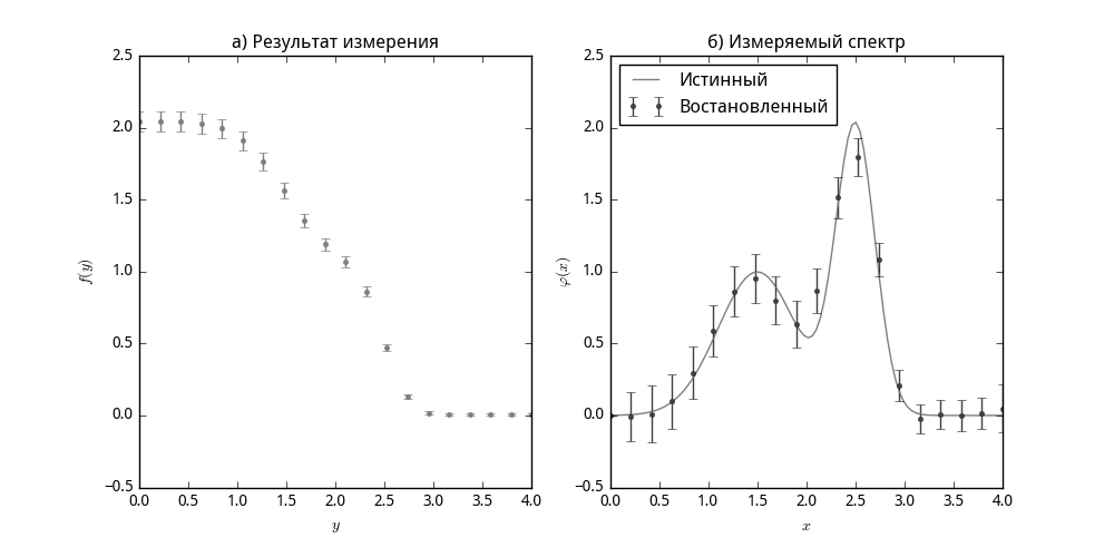
As an example, we consider the reconstruction of a spectrum consisting of two Gaussian peaks that fell under the action of an integral step kernel (Heaviside function).